Weather data and solar radiation on a tilted surface#
![]()
Introduction#
Objectives#
Download weather data in EnergyPlus™ format.
Read weather data.
Find solar radiation on a tilted surface.
Visualize the data.
Summary#
This notebook:
Imports standard modules such as
numpy,pandas, andmatplotlib.pyplot, and a local (dedicated) module, dm4bem and reads the file FRA_Lyon.074810_IWEC.epw in EnergyPlus™ Weather Format (.epw) containing weather data for Lyon, France.Selects three columns from the weather data, namely air temperature, direct radiation on a normal surface, and diffuse radiation on an horizontal surface, and replaces with 2000 the years in the index of the dataframe.
Defines a start date and an end date and filters the weather data based on these dates.
Creates three line plots using the filtered weather data:
Outdoor air temperature over time.
Solar radiation (normal direct and horizontal diffuse) over time.
Solar radiation on a tilted surface over time, calculated using the filtered weather data and the slope, azimuth, and latitude of the surface.
Calculates the solar radiation on a tilted surface by computing the direct radiation, diffuse radiation, and reflected radiation. It then stores the calculated solar radiation as a new column in the filtered weather data.
Obtain weather data in EnergyPlus™ format#
import numpy as np
import pandas as pd
import matplotlib.pyplot as plt

from dm4bem import read_epw, sol_rad_tilt_surf
Download data file#
Download the weather file with extension .epw from:
Climate.OneBuilding.Org: repository of free climate data for building performance simulation,
EnergyPlus™: interactive map with locations,
LadyBug Tools: interactive map with locations,
PV GIS: interactive map with interpolated data.
For example, for the airport Lyon-Bron, France (N45.73, E5.08), download the files:
from Climate OneBuilding and place them in the ./weather_data folder
or, from PV GIS, select a location on the interactive map and dowload TMY (Typical Meteorological Year) data in .epwformat.
Read weather data#
Weather data file name#
filename = '../weather_data/FRA_Lyon.074810_IWEC.epw'
# filename = '../weather_data/FRA_AR_Lyon-Bron.AP.074800_TMYx.2004-2018.epw'
The weather file .epw contains hourly data for one year. For the description of the structure and the meaning of the fields of the .epw file, see read_epw function in dm4bem.py module and the documentation for pvlib.iotools.read_epw function of pvlib python.
[data, meta] = read_epw(filename, coerce_year=None)
data
| year | month | day | hour | minute | data_source_unct | temp_air | temp_dew | relative_humidity | atmospheric_pressure | ... | ceiling_height | present_weather_observation | present_weather_codes | precipitable_water | aerosol_optical_depth | snow_depth | days_since_last_snowfall | albedo | liquid_precipitation_depth | liquid_precipitation_quantity | |
|---|---|---|---|---|---|---|---|---|---|---|---|---|---|---|---|---|---|---|---|---|---|
| 1983-01-01 00:00:00+01:00 | 1983 | 1 | 1 | 1 | 60 | C9C9C9C9*0?9?9?9?9?9?9?9A7A7A7A7A7A7*0E8*0*0 | 0.8 | 0.3 | 96 | 100100 | ... | 15 | 0 | 999999599 | 0 | 0.204 | 0 | 88 | 0.0 | 0.0 | 0.0 |
| 1983-01-01 01:00:00+01:00 | 1983 | 1 | 1 | 2 | 60 | C9C9C9C9*0?9?9?9?9?9?9?9A7A7B8B8A7A7*0E8*0*0 | -0.6 | -0.9 | 97 | 100300 | ... | 30 | 0 | 999999599 | 0 | 0.204 | 0 | 88 | 0.0 | 0.0 | 0.0 |
| 1983-01-01 02:00:00+01:00 | 1983 | 1 | 1 | 3 | 60 | C9C9C9C9*0?9?9?9?9?9?9?9A7A7B8B8A7A7*0E8*0*0 | -1.5 | -1.7 | 98 | 100400 | ... | 30 | 0 | 999999599 | 0 | 0.204 | 0 | 88 | 0.0 | 0.0 | 0.0 |
| 1983-01-01 03:00:00+01:00 | 1983 | 1 | 1 | 4 | 60 | C9C9C9C9*0?9?9?9?9?9?9?9A7A7A7A7A7A7*0E8*0*0 | -1.9 | -2.0 | 99 | 100500 | ... | 30 | 0 | 999999599 | 0 | 0.204 | 0 | 88 | 0.0 | 0.0 | 0.0 |
| 1983-01-01 04:00:00+01:00 | 1983 | 1 | 1 | 5 | 60 | C9C9C9C9*0?9?9?9?9?9?9?9A7A7B8B8A7A7*0E8*0*0 | -2.1 | -2.2 | 100 | 100500 | ... | 30 | 0 | 999999599 | 0 | 0.204 | 0 | 88 | 0.0 | 0.0 | 0.0 |
| ... | ... | ... | ... | ... | ... | ... | ... | ... | ... | ... | ... | ... | ... | ... | ... | ... | ... | ... | ... | ... | ... |
| 1986-12-31 19:00:00+01:00 | 1986 | 12 | 31 | 20 | 60 | C9C9C9C9*0?9?9?9?9?9?9?9A7A7B8B8A7A7*0E8*0*0 | 5.9 | 4.7 | 92 | 99400 | ... | 22000 | 9 | 999999999 | 0 | 0.117 | 2 | 88 | 0.0 | 0.0 | 0.0 |
| 1986-12-31 20:00:00+01:00 | 1986 | 12 | 31 | 21 | 60 | C9C9C9C9*0?9?9?9?9?9?9?9A7A7B8B8A7A7*0E8*0*0 | 5.5 | 4.5 | 93 | 99400 | ... | 22000 | 9 | 999999999 | 0 | 0.117 | 2 | 88 | 0.0 | 0.0 | 0.0 |
| 1986-12-31 21:00:00+01:00 | 1986 | 12 | 31 | 22 | 60 | C9C9C9C9*0?9?9?9?9?9?9?9A7A7A7A7A7A7*0E8*0*0 | 4.9 | 3.9 | 94 | 99500 | ... | 22000 | 9 | 999999999 | 0 | 0.117 | 2 | 88 | 0.0 | 0.0 | 0.0 |
| 1986-12-31 22:00:00+01:00 | 1986 | 12 | 31 | 23 | 60 | C9C9C9C9*0?9?9?9?9?9?9?9A7A7B8B8A7A7*0E8*0*0 | 3.7 | 2.9 | 94 | 99600 | ... | 22000 | 9 | 999999999 | 0 | 0.117 | 2 | 88 | 0.0 | 0.0 | 0.0 |
| 1986-12-31 23:00:00+01:00 | 1986 | 12 | 31 | 24 | 60 | C9C9C9C9*0?9?9?9?9?9?9?9A7A7B8B8A7A7*0E8*0*0 | 2.3 | 1.6 | 95 | 99800 | ... | 1320 | 9 | 999999999 | 0 | 0.117 | 2 | 88 | 0.0 | 0.0 | 0.0 |
8760 rows × 35 columns
Weather data is from different years#
The weather data from Climate One Buildings are Typical Meteorological Years (TMY). Therefore, data for each month is from different years.
# Extract the month and year from the DataFrame index with the format 'MM-YYYY'
month_year = data.index.strftime('%m-%Y')

# Create a set of unique month-year combinations
unique_month_years = sorted(set(month_year))

# Create a DataFrame from the unique month-year combinations
pd.DataFrame(unique_month_years, columns=['Month-Year'])
| Month-Year | |
|---|---|
| 0 | 01-1983 |
| 1 | 02-1985 |
| 2 | 03-1998 |
| 3 | 04-1995 |
| 4 | 05-1986 |
| 5 | 06-1993 |
| 6 | 07-1982 |
| 7 | 08-1993 |
| 8 | 09-1988 |
| 9 | 10-1999 |
| 10 | 11-1991 |
| 11 | 12-1986 |
From the dataset, select:
EPW Data field |
Mean during 1 h prior to timestamp |
Unit |
|---|---|---|
|
Dry bulb air temperature |
°C |
|
Direct normal radiation |
W·m⁻² |
|
Diffuse horizontal radiation |
W·m⁻² |
Note: For the description of .epw file, see pvlib.iotools.epw.
Since the values for each month are from different years, let’s replace the different years with the same year, e.g. 2000.
# select columns of interest
weather_data = data[["temp_air", "dir_n_rad", "dif_h_rad"]]

# replace year with 2000 in the index
weather_data.index = weather_data.index.map(
    lambda t: t.replace(year=2000))
Let’s check the weather data at a given date and time.
weather_data.loc['2000-06-29 12:00']
temp_air      25.7
dir_n_rad    204.0
dif_h_rad    423.0
Name: 2000-06-29 12:00:00+01:00, dtype: float64
Start and end time#
Select a period for:
air temperature, °C,
normal solar radiation, W·m⁻²,
mean diffuse solar radiation received during 60 minutes prior to timestamp, W·m⁻².
# Define start and end dates
start_date = '2000-06-29 12:00'
end_date = '2000-07-02'         # time is 00:00 if not indicated

# Filter the data based on the start and end dates
weather_data = weather_data.loc[start_date:end_date]
del data
weather_data
| temp_air | dir_n_rad | dif_h_rad | |
|---|---|---|---|
| 2000-06-29 12:00:00+01:00 | 25.7 | 204 | 423 |
| 2000-06-29 13:00:00+01:00 | 26.0 | 227 | 439 |
| 2000-06-29 14:00:00+01:00 | 26.0 | 265 | 407 |
| 2000-06-29 15:00:00+01:00 | 24.7 | 312 | 335 |
| 2000-06-29 16:00:00+01:00 | 19.0 | 166 | 294 |
| ... | ... | ... | ... |
| 2000-07-02 19:00:00+01:00 | 25.0 | 0 | 19 |
| 2000-07-02 20:00:00+01:00 | 24.0 | 0 | 2 |
| 2000-07-02 21:00:00+01:00 | 24.0 | 0 | 0 |
| 2000-07-02 22:00:00+01:00 | 24.0 | 0 | 0 |
| 2000-07-02 23:00:00+01:00 | 22.0 | 0 | 0 |
84 rows × 3 columns
Plot outdoor air temperature#
weather_data['temp_air'].plot()
plt.xlabel("Time")
plt.ylabel("Dry-bulb air temperature, θ / °C")
plt.legend([])
plt.show()
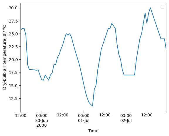
Figure 1. Hourly dry bulb air temperature at timestamp.
Plot solar radiation: normal direct and horizontal diffuse#
weather_data[['dir_n_rad', 'dif_h_rad']].plot()
plt.xlabel("Time")
plt.ylabel("Solar radiation, Φ / (W·m⁻²)")
plt.legend(['$Φ_{direct}$', '$Φ_{diffuse}$'])
plt.show()
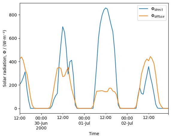
Figure 2. Hourly-mean direct normal and difuse horizontal solar radiation.
Solar radiation on a tilted surface#
Orientation of the tilted wall#
Knowing the albedo of the surface which is in front of a tilted wall, the diffuse and reflected radiation incident on the wall can be calculated from weather data for each hour.
Let’s consider a wall at latitude \(\phi\) with the orientation given by its slope angle, \(\beta\), and azimuth angle, \(\gamma\).
surface_orientation = {'slope': 90,     # 90° is vertical; > 90° downward
                       'azimuth': 0,    # 0° South, positive westward
                       'latitude': 45}  # °, North Pole 90° positive

Figure 3. Orientation of a surface:
\(\beta\): slope angle: \(\beta = 90°\) is vertical; \(\beta > 90°\) is downward facing.
\(\gamma\): azimuth angle: 0° South, positive westward, negative eastward.
\(\theta\): incidence angle: angle between the solar beam on the surface and the normal to the surface.
N, S, E, W: North, South, East and West, respectively. \(\vec{n}\) is the vector normal to the surface. ∟ represents right angles.
Let’s consider that the albedo of the surface in front of the wall is known.
albedo = 0.2
Plot the solar radiation#
rad_surf = sol_rad_tilt_surf(
    weather_data, surface_orientation, albedo)

rad_surf.plot()
plt.xlabel("Time")
plt.ylabel("Solar irradiance,  Φ / (W·m⁻²)")
plt.show()
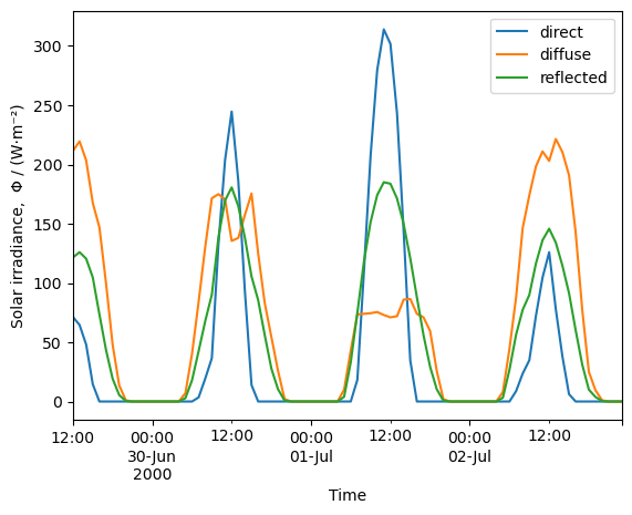
Figure 4. Hourly-mean direct, diffuse and reflected irradiance on a tilted surface.
The values of solar irradiance can be obtained for a specific date and time.
print(f"{rad_surf.loc['2000-06-29 12:00']['direct']:.0f} W/m²")
71 W/m²
Statistics, such as mean and maximum value, can be calculated.
print(f"Mean. direct irradiation: {rad_surf['direct'].mean():.0f} W/m²")
print(f"Max. direct irradiation:  {rad_surf['direct'].max():.0f} W/m²")
Mean. direct irradiation: 39 W/m²
Max. direct irradiation:  314 W/m²
print(f"Direct solar irradiance is maximum on {rad_surf['direct'].idxmax()}")
Direct solar irradiance is maximum on 2000-07-01 11:00:00+01:00
Calculation of solar radiation on a tilted surface from weather data#
Let’s consider a tilted surface having another surface (e.g., ground) in front of it. Given the weather data, the surface orientation, and the albedo of the ground in front of the surface, find the direct, diffuse and reflected solar radiation for this surface. The algoritm is implemented in the function sol_rad_tilt_surf of the dm4bem.py module.
Surface orientation#
The orientation of the surface is given by the following angles (Duffie et al. (2020), p.13):
\(\beta\) slope: slope or tilt angle from 0 to 180 degrees
β = 0° - horizontal, upward facing;
β = 90°- vertical;
β < 90°- upward facing;
β > 90°- downward facing;
180° - horizontal, downward facing.
\(\gamma\) azimuth: surface azimuth in degrees, \(-180 ^{\circ} \leq \gamma \leq 180 ^{\circ}\); 0-south; westward: positive; eastward: negatif.
\(\phi\) latitude: local latitude in degree \(-90 ^{\circ} \leq \phi \leq 90 ^{\circ}\); northward: positive, southward: negative.
β = surface_orientation['slope']
γ = surface_orientation['azimuth']
ϕ = surface_orientation['latitude']

# Transform degrees in radians
β = β * np.pi / 180
γ = γ * np.pi / 180
ϕ = ϕ * np.pi / 180

n = weather_data.index.dayofyear
Total solar radiation is the amount of radiation received on a surface during the number of minutes preceding the time indicated:
where:
\(G_{dir}\) direct normal or beam radiation: amount of solar radiation received directly from the solar disk on a surface perpendicular to the sun’s rays, during the number of minutes preceding the time indicated, W/m².
\(G_{dif}\) diffuse radiation: amount of solar radiation received after scattering by the atmosphere, W/m². It does not include the diffuse infrared radiation emitted by the atmosphere, W/m².
\(G_r\) total solar radiation coming by reflection from the surface in front of the wall (usually, ground), W/m².
Direct radiation#
The direct radiation on the surface, \(G_{dir}\), depends on the direct normal (or beam) radiation, \(G_n\), and the incidence angle, \(\theta\), between the solar beam and the normal to the wall (Réglementation Thermique 2005, §11.2.1).
In order to calculate the incidence angle, \(\theta\), we need:
\(\phi\) latitude, the angle between the position and the Equator, ranging from 0° at the Equator to 90° at the North Pole and -90° at the South Pole. \(-90 ^{\circ} \leq \phi \leq 90 ^{\circ}\)
\(\beta\) slope, the angle between the plane of the surface and the horizontal. \(0 \le \beta \le 180 ^{\circ}\). If \(\beta = 0 ^{\circ}\), the surface is horizontal, upward facing; if \(0^{\circ} < \beta < 90^{\circ}\), the surface is upward facing; if \(\beta = 90 ^{\circ}\), the surface is vertical.
\(\gamma\) azimuth, the angle between the projection on a horizontal plane of the normal to the surface and the local meridian; south is zero, east negative, and west positive. \(-180 ^{\circ} \leq \gamma \leq 180 ^{\circ}\).
\(\delta\) declination angle, the angle between the sun at noon (i.e., when the sun is on the local meridian) and the plane of the equator, north positive (Duffie et al. 2020, eq. 1.6.1a, p. 14, Réglementation Thermique 2005 §11.2.1.1, eq. (78)):
declination_angle = 23.45 * np.sin(360 * (284 + n) / 365 * np.pi / 180)
δ = declination_angle * np.pi / 180
\(\omega\) solar hour angle, the angle between the sun and the local meridian due to rotation of the earth around its axis at 15° per hour (Duffie et al. 2020, p.13):
where hour and minute is the solar time.
Note: \(-180 ^{\circ} \leq \omega \leq 180 ^{\circ}\). \(\omega < 0\) in the morning, \(\omega = 0\) at noon, and \(\omega > 0\) in the afternoon. Hour angle is used with the declination to give the direction of a point on the celestial sphere.
hour = weather_data.index.hour
minute = weather_data.index.minute + 60
hour_angle = 15 * ((hour + minute / 60) - 12)   # deg
ω = hour_angle * np.pi / 180                    # rad
The incidence angle, \(\theta\), is the angle between the solar beam on the surface and the normal to the surface (Duffie et al. 2020, eq. 1.6.2, p. 14):
If \(\beta \le 90^\circ\), then the sun is behind the surface. Therefore, if \(\theta > \pi / 2\), then \(\theta = \pi / 2\).
theta = np.sin(δ) * np.sin(ϕ) * np.cos(β) \
    - np.sin(δ) * np.cos(ϕ) * np.sin(β) * np.cos(γ) \
    + np.cos(δ) * np.cos(ϕ) * np.cos(β) * np.cos(ω) \
    + np.cos(δ) * np.sin(ϕ) * np.sin(β) * np.cos(γ) * np.cos(ω) \
    + np.cos(δ) * np.sin(β) * np.sin(γ) * np.sin(ω)

theta = np.array(np.arccos(theta))
theta = np.minimum(theta, np.pi / 2)
The direct radiation, \(G_{dir}\) on the surface is:
where direct normal radiation or beam radiation, \(G_n\), is the amount of solar radiation (in W/m²) received directly from the solar disk on the surface perpendicular to the sun’s rays during the number of minutes preceding the time indicated. It is given by weather data.
dir_rad = weather_data["dir_n_rad"] * np.cos(theta)
dir_rad[dir_rad < 0] = 0
Diffuse radiation#
The diffuse radiation on the wall is a function of its slope, \(\beta\), and the isotropic diffuse solar radiation, \(G_{dif,h}\), (Réglementation thermique 2005, §1.2.1.2, eq. 79, p. 31):
Note: \(\forall \beta, \frac{1 + \cos \beta}{2} \geq 0.\)
dif_rad = weather_data["dif_h_rad"] * (1 + np.cos(β)) / 2
Solar radiation reflected by the ground#
Considering the radiation reflected by the ground as isotropic, the reflected radiation that gets onto the wall is a function of its slope, albedo and total horizontal radiation (Réglementation Thermique 2005, §11.2.1.3).
The normal horizontal radiation is (Réglementation Thermique 2005 eq. 80):
gamma = np.cos(δ) * np.cos(ϕ) * np.cos(ω) \
    + np.sin(δ) * np.sin(ϕ)

gamma = np.array(np.arcsin(gamma))
gamma[gamma < 1e-5] = 1e-5

dir_h_rad = weather_data["dir_n_rad"] * np.sin(gamma)
The total radiation received by reflection is:
where \(\rho\) is the albedo (or the reflection coefficient) of the surface and \(\beta\) is the slope of the surface.
Note: \(\forall \beta, \frac{1 - \cos \beta}{2} \geq 0.\)
ref_rad = (dir_h_rad + weather_data["dif_h_rad"]) * albedo \
        * (1 - np.cos(β) / 2)
Definitions#
Radiation and time#
\(G_{dir,n}\) Direct normal or beam radiation. Amount of solar radiation in Wh/m² received directly from the solar disk on a surface perpendicular to the sun’s rays, during the number of minutes preceding the time indicated.
\(G_{dif,h}\) Diffuse horizontal radiation. Amount of solar radiation in Wh/m² received after scattering by the atmosphere. This definition distinguishes the diffuse solar radiation from infrared radiation emitted by the atmosphere.
Total Solar Radiation. Total amount of direct and diffuse solar radiation in Wh/m² received on a surface during the number of minutes preceding the time indicated.
Global radiation. Total solar radiation given on a horizontal surface.
Solar Time. Time based on the apparent position of the sun in the sky with noon the time when the sun crosses the observer meridian.
Definitions for angles (in degrees)#
\(\phi\) Latitude. Angle between the position and the Equator, ranging from 0° at the Equator to 90° at the North Pole and -90° at the South Pole. \(-90 ^{\circ} \leq \phi \leq 90 ^{\circ}\)
\(\beta\) Slope. Angle between the plane of the surface and the horizontal. \(\beta = 0\) means that the surface is horizontal, upward facing; \(0 \le \beta \le 180 ^{\circ}\). \(\beta < 90^{\circ}\) means that the surface is upward facing; \(\beta = 90^{\circ}\) the surface is vertical.
\(\gamma\) Azimuth. Angle between the projection on a horizontal plane of the normal to the surface and the local meridian; south is zero, east negative, and west positive. \(-180 ^{\circ} \leq \gamma \leq 180^{\circ}\).
\(\delta\) Declination. Angle between the sun at noon (i.e., when the sun is on the local meridian) and the plane of the equator, north positive (Duffie et al. 2020, eq. 1.6.1a):
where \(n\) is the day of the year. \(-23.45 ^{\circ} \leq \delta \leq 23.45 ^{\circ}\). Declination is used with hour angle to give the direction of a point on the celestial sphere.
\(\omega\) Hour angle. Angle between the sun and the local meridian due to rotation of the earth around its axis at 15° per hour (Duffie et al. 2020, Example 1.6.1 p.15):
where \(h\) and \(min\) are hours and and minutes of the solar time, respectively. The hour angle is \(-180 ^{\circ} \leq \omega \leq 180 ^{\circ}\), with \(\omega < 0\) in the morning, \(\omega = 0\) at noon, and \(\omega > 0\) in the afternoon. Hour angle is used with the declination to give the direction of a point on the celestial sphere.
\(\theta\) Incidence. Angle between the solar beam on the surface and the normal to the surface (Duffie et al. 2020, eq. 1.6.2):
References#
Duffie, J.A., Beckman, W. A., Blair, N. (2020) Solar Engineering of Thermal Processes, 5th ed. John Wiley & Sons, Inc. ISBN 9781119540281
Réglementation Thermique 2005. Méthode de calcul Th-CE. Annexe à l’arrêté du 19 juillet 2006
US Department of Energy (2022) EnergyPlus™ Engineering Reference, version 22.1.0, © 1996-2022