Simulation: perfect controller#
![]()
The simulation is done by numerical integration of the state-space representation by using the description of the model as a thermal circuit, the input data set, and the weather data.
Objectives:
Resample the inputs at time step.
Create input vector in time.
Integrate in time the state-space model.
Plot the results.
import numpy as np
import pandas as pd
import matplotlib.pyplot as plt
import control as ctrl
import time

import dm4bem
The following assumptions can be done (see Figure 1):
The indoor air temperature is not controlled (i.e., the building is in free running) or it is controlled by a P-controller having the gain \(K_p = G_{11}.\)
The capacities of the air, \(C_6\), and of the glass, \(C_7\), can be neglected or not.
The time integration is done by using Euler explicit or Euler implicit.
The time step is calculated from the eigenvalues of the state matrix or it is imposed at a value designated as \(\Delta t\).

Figure 1. Thermal circuit for the cubic building.
controller = True
Kp = 1e3    # W/°C, controller gain

neglect_air_capacity = False
neglect_glass_capacity = False

explicit_Euler = True

imposed_time_step = False
Δt = 3600    # s, imposed time step
State-space representation#
The thermal circuit was described in the section on modelling. It is read from the file ./toy_model/TC.csv. Thermal circuit is transformed in state-space representation.
# MODEL
# =====
# Thermal circuits
TC = dm4bem.file2TC('./toy_model/TC.csv', name='', auto_number=False)

# by default TC['G']['q11'] = 0 # Kp -> 0, no controller (free-floating
if controller:
    TC['G']['q11'] = Kp     # G11 = Kp, conductance of edge q11
                            # Kp -> ∞, almost perfect controller
if neglect_air_capacity:
    TC['C']['θ6'] = 0       # C6, capacity of vertex θ6 (air)
if neglect_glass_capacity:
    TC['C']['θ7'] = 0       # C7, capacity of vertex θ7 (glass)

# State-space
[As, Bs, Cs, Ds, us] = dm4bem.tc2ss(TC)
dm4bem.print_TC(TC)
A:
      θ0   θ1   θ2   θ3   θ4   θ5   θ6   θ7
q0   1.0  0.0  0.0  0.0  0.0  0.0  0.0  0.0
q1  -1.0  1.0  0.0  0.0  0.0  0.0  0.0  0.0
q2   0.0 -1.0  1.0  0.0  0.0  0.0  0.0  0.0
q3   0.0  0.0 -1.0  1.0  0.0  0.0  0.0  0.0
q4   0.0  0.0  0.0 -1.0  1.0  0.0  0.0  0.0
q5   0.0  0.0  0.0  0.0 -1.0  1.0  0.0  0.0
q6   0.0  0.0  0.0  0.0 -1.0  0.0  1.0  0.0
q7   0.0  0.0  0.0  0.0  0.0 -1.0  1.0  0.0
q8   0.0  0.0  0.0  0.0  0.0  0.0  0.0  1.0
q9   0.0  0.0  0.0  0.0  0.0  1.0  0.0 -1.0
q10  0.0  0.0  0.0  0.0  0.0  0.0  1.0  0.0
q11  0.0  0.0  0.0  0.0  0.0  0.0  1.0  0.0

G:
q0     1125.000000
q1      630.000000
q2      630.000000
q3       30.375000
q4       30.375000
q5       44.786824
q6      360.000000
q7       72.000000
q8      165.789474
q9      630.000000
q10       9.000000
q11    1000.000000
Name: G, dtype: float64

C:
θ0           0.0
θ1    18216000.0
θ2           0.0
θ3      239580.0
θ4           0.0
θ5           0.0
θ6       32400.0
θ7     1089000.0
Name: C, dtype: float64

b:
q0        To
q1         0
q2         0
q3         0
q4         0
q5         0
q6         0
q7         0
q8        To
q9         0
q10       To
q11    Ti_sp
Name: b, dtype: object

f:
θ0     Φo
θ1    0.0
θ2    0.0
θ3    0.0
θ4     Φi
θ5    0.0
θ6     Qa
θ7     Φa
Name: f, dtype: object

y:
θ0    0.0
θ1    0.0
θ2    0.0
θ3    0.0
θ4    0.0
θ5    0.0
θ6    1.0
θ7    0.0
Name: y, dtype: float64
The condition for numerical stability of Euler explicit integration,
where \(\lambda_i\) are the eigenvalues of the state matrix, gives the time step used in numerical integration.
λ = np.linalg.eig(As)[0]    # eigenvalues of matrix As
dtmax = 2 * min(-1. / λ)    # max time step for Euler explicit stability
dt = dm4bem.round_time(dtmax)

if imposed_time_step:
    dt = Δt

dm4bem.print_rounded_time('dt', dt)
dt = 50 s
Input data set#
One-hour time step#
The input data set was described in the section on inputs. It is at the sampling time of 1 h (according to the weather file .epw, see notebook on Inputs).
# INPUT DATA SET
# ==============
input_data_set = pd.read_csv('./toy_model/input_data_set.csv',
                             index_col=0,
                             parse_dates=True)
input_data_set
| To | Ti_sp | Φo | Φi | Qa | Φa | Etot | |
|---|---|---|---|---|---|---|---|
| 2000-02-01 12:00:00+01:00 | 10.0 | 20 | 803.250000 | 146.341093 | 0.0 | 244.188000 | 71.400000 |
| 2000-02-01 13:00:00+01:00 | 11.0 | 20 | 787.500000 | 143.471660 | 0.0 | 239.400000 | 70.000000 |
| 2000-02-01 14:00:00+01:00 | 13.0 | 20 | 3392.970859 | 618.152586 | 0.0 | 1031.463141 | 301.597410 |
| 2000-02-01 15:00:00+01:00 | 11.0 | 20 | 456.750000 | 83.213563 | 0.0 | 138.852000 | 40.600000 |
| 2000-02-01 16:00:00+01:00 | 11.0 | 20 | 378.000000 | 68.866397 | 0.0 | 114.912000 | 33.600000 |
| ... | ... | ... | ... | ... | ... | ... | ... |
| 2000-02-07 14:00:00+01:00 | 6.0 | 20 | 1794.968843 | 327.018615 | 0.0 | 545.670528 | 159.552786 |
| 2000-02-07 15:00:00+01:00 | 6.0 | 20 | 1616.246876 | 294.457933 | 0.0 | 491.339050 | 143.666389 |
| 2000-02-07 16:00:00+01:00 | 6.0 | 20 | 611.793325 | 111.460322 | 0.0 | 185.985171 | 54.381629 |
| 2000-02-07 17:00:00+01:00 | 5.0 | 20 | 78.750000 | 14.347166 | 0.0 | 23.940000 | 7.000000 |
| 2000-02-07 18:00:00+01:00 | 4.2 | 20 | 0.000000 | 0.000000 | 0.0 | 0.000000 | 0.000000 |
151 rows × 7 columns
Resample input data set#
The weather data and the scheduled sources are at the time-step of 1 h. The data needs to be resampled at time step dt used for numerical integration.
input_data_set = input_data_set.resample(
    str(dt) + 'S').interpolate(method='linear')
input_data_set.head()
| To | Ti_sp | Φo | Φi | Qa | Φa | Etot | |
|---|---|---|---|---|---|---|---|
| 2000-02-01 12:00:00+01:00 | 10.000000 | 20.0 | 803.25000 | 146.341093 | 0.0 | 244.1880 | 71.400000 |
| 2000-02-01 12:00:50+01:00 | 10.013889 | 20.0 | 803.03125 | 146.301240 | 0.0 | 244.1215 | 71.380556 |
| 2000-02-01 12:01:40+01:00 | 10.027778 | 20.0 | 802.81250 | 146.261387 | 0.0 | 244.0550 | 71.361111 |
| 2000-02-01 12:02:30+01:00 | 10.041667 | 20.0 | 802.59375 | 146.221533 | 0.0 | 243.9885 | 71.341667 |
| 2000-02-01 12:03:20+01:00 | 10.055556 | 20.0 | 802.37500 | 146.181680 | 0.0 | 243.9220 | 71.322222 |
Input vector in time#
In the input data set an input, e.g. \(T_o\), appears only once. However, the i nput vector may contain the same time series multiple time; for example, in the model presented in Figure 1, there are three inputs \(T_o\) corresponding to branches \(q_0\), \(q_8\), and \(q_{10}\)). Therefore, we need to obtain the input vector from the input data set.
The input in time is formed by the vectors of time series of temperature sources \(\left [ T_o, T_o ,T_o, T_{i,sp} \right ]^T\) and vectors of time series of the heat flow sources \(\left [ \Phi_o, \Phi_i, \dot{Q_a}, \Phi_a \right ]^T\):
where the input data set is:
\(T_o\): the time series vector of outdoor temperatures (from weather data), °C.
\(T_{i,sp}\): time series vector of indoor setpoint temperatures, °C.
\(\Phi_o\): time series vector of solar (i.e. short wave) radiation absorbed by the outdoor surface of the wall, W;
\(\Phi_i\): time series vector of short wave (i.e. solar) radiation absorbed by the indoor surfaces of the wall, W;
\(\dot{Q}_a\): time vector of auxiliary heat flows (from occupants, electrical devices, etc.), W.
\(\Phi_a\): time series vector of short wave (i.e. solar) radiation absorbed by the window glass, W.
The input vector u is obtained from the input data set, \(T_o, T_{i,sp}, \Phi_o, \Phi_i, \dot Q_a, \Phi_a\), by using the order of the sources given in the state-space model, us: q0 = \(T_o\), q8 = \(T_o\), q10 = \(T_o\), q11 = \(T_{i,sp}\), θ0 = \(\Phi_o\), θ4 = \(\Phi_i\), θ6 = \(\dot Q_a\), and θ7 = \(\Phi_a\).
# Input vector in time from input_data_set
u = dm4bem.inputs_in_time(us, input_data_set)
u.head()
| q0 | q8 | q10 | q11 | θ0 | θ4 | θ6 | θ7 | |
|---|---|---|---|---|---|---|---|---|
| 2000-02-01 12:00:00+01:00 | 10.000000 | 10.000000 | 10.000000 | 20.0 | 803.25000 | 146.341093 | 0.0 | 244.1880 |
| 2000-02-01 12:00:50+01:00 | 10.013889 | 10.013889 | 10.013889 | 20.0 | 803.03125 | 146.301240 | 0.0 | 244.1215 |
| 2000-02-01 12:01:40+01:00 | 10.027778 | 10.027778 | 10.027778 | 20.0 | 802.81250 | 146.261387 | 0.0 | 244.0550 |
| 2000-02-01 12:02:30+01:00 | 10.041667 | 10.041667 | 10.041667 | 20.0 | 802.59375 | 146.221533 | 0.0 | 243.9885 |
| 2000-02-01 12:03:20+01:00 | 10.055556 | 10.055556 | 10.055556 | 20.0 | 802.37500 | 146.181680 | 0.0 | 243.9220 |
Initial conditions#
The initial value of the state-vector can be zero or different from zero.
# Initial conditions
θ0 = 20.0                   # °C, initial temperatures
θ = pd.DataFrame(index=u.index)
θ[As.columns] = θ0          # fill θ with initial valeus θ0
Time integration#
The state-space model
is integrated in time by using Euler forward (or explicit) method for numerical integration:
or Euler backward (or implicit) method for numerical integration:
where \(k = 0, ... , n - 1\).
I = np.eye(As.shape[0])     # identity matrix

if explicit_Euler:
    for k in range(u.shape[0] - 1):
        θ.iloc[k + 1] = (I + dt * As) @ θ.iloc[k] + dt * Bs @ u.iloc[k]
else:
    for k in range(u.shape[0] - 1):
        θ.iloc[k + 1] = np.linalg.inv(
            I - dt * As) @ (θ.iloc[k] + dt * Bs @ u.iloc[k])
Outputs#
From the time variation of state variable \(\theta_s\) we obtain the time variation of the output \(y\) (i.e., indoor temperature):
# outputs
y = (Cs @ θ.T + Ds @  u.T).T
and the variation in time of the heat flow of the HVAC system:
where \(K_p\) is the gain of the P-controller and \(T_{i,sp}\) is the HVAC-setpoint for the indoor temperature.
Kp = TC['G']['q11']     # controller gain
S = 9                   # m², surface area of the toy house
q_HVAC = Kp * (u['q11'] - y['θ6']) / S  # W/m²
y['θ6']
2000-02-01 12:00:00+01:00    20.000000
2000-02-01 12:00:50+01:00    20.051355
2000-02-01 12:01:40+01:00    20.004418
2000-02-01 12:02:30+01:00    20.030324
2000-02-01 12:03:20+01:00    20.002447
                               ...
2000-02-07 17:56:40+01:00    18.921625
2000-02-07 17:57:30+01:00    18.920398
2000-02-07 17:58:20+01:00    18.919173
2000-02-07 17:59:10+01:00    18.917951
2000-02-07 18:00:00+01:00    18.916731
Freq: 50S, Name: θ6, Length: 10801, dtype: float64
Plots#
We select the data to plot:
\(T_o\), outdoor temperature, °C;
\(\theta_i\), indoor temperature, °C;
\(E_{tot}\), total solar irradiance, W/m²;
\(q_{HVAC}\), thermal load, i.e., the power that the HVAC system needs to deliver in order to maintain the indoor air temperature at its set-point, W.
data = pd.DataFrame({'To': input_data_set['To'],
                     'θi': y['θ6'],
                     'Etot': input_data_set['Etot'],
                     'q_HVAC': q_HVAC})
Plots using Pandas#
The plots mays be done by using plot method for DataFrame.
fig, axs = plt.subplots(2, 1)
data[['To', 'θi']].plot(ax=axs[0],
                        xticks=[],
                        ylabel='Temperature, $θ$ / °C')

axs[0].legend(['$θ_{outdoor}$', '$θ_{indoor}$'],
              loc='upper right')

data[['Etot', 'q_HVAC']].plot(ax=axs[1],
                              ylabel='Heat rate, $q$ / (W·m⁻²)')
axs[1].set(xlabel='Time')
axs[1].legend(['$E_{total}$', '$q_{HVAC}$'],
              loc='upper right')
plt.show();
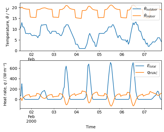
Figure 2. Simulation in free-running with weather data using Euler explicit method of integration. a) Indoor and outdoor temperatures. b) Solar and HVAC heat flow rates.
Plots using matplotlib#
Alternatively, we may use matplotlib.
t = dt * np.arange(data.shape[0])   # time vector

fig, axs = plt.subplots(2, 1)
# plot outdoor and indoor temperature
axs[0].plot(t / 3600 / 24, data['To'], label='$θ_{outdoor}$')
axs[0].plot(t / 3600 / 24, y.values, label='$θ_{indoor}$')
axs[0].set(ylabel='Temperatures, $θ$ / °C',
           title='Simulation for weather')
axs[0].legend(loc='upper right')

# plot total solar radiation and HVAC heat flow
axs[1].plot(t / 3600 / 24, data['Etot'], label='$E_{total}$')
axs[1].plot(t / 3600 / 24, q_HVAC, label='$q_{HVAC}$')
axs[1].set(xlabel='Time, $t$ / day',
           ylabel='Heat flows, $q$ / (W·m⁻²)')
axs[1].legend(loc='upper right')

fig.tight_layout()
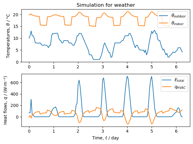
Figure 3. Simulation in free-running with weather data using Euler explicit method of integration. a) Indoor and outdoor temperatures. b) Solar and HVAC heat flow rates.
Discussion#
Numerical integration method#
While fixed-step methods like Euler explicit or implicit integration can be simpler to implement and understand, they may not be the most efficient choice. Variable time step methods offer greater adaptability and efficiency, making them preferable for many simulation scenarios.
Let’s compare the simulation time by using Euler explicit and variable time step used in Python Control Systems Library.
The use of Euler numerical integration method is justified when the input vector varies during the numerical integration and changes are done in the for loop.
sys = ctrl.ss(As, Bs, Cs, Ds)

θ0 = 20.0 * np.ones(As.shape[0])  # °C, initial temperatures
The convention used by Python Control Systems Library for time series is different from the convention used in Pandas and scipy.signal library: columns represent different points in time, rows are different components (e.g., inputs, outputs or states). Since dm4bem uses Pandas, the vector of inputs in time must be transposed.
u_np = u.values.T # inputs in time
start_time = time.time()

# Simulate the system response with Python Control Systems Library
t, yout = ctrl.input_output_response(sys, T=t, U=u_np, X0=θ0)

end_time = time.time()
duration_1 = end_time - start_time
start_time = time.time()

# Euler explicit
for k in range(u.shape[0] - 1):
    θ.iloc[k + 1] = (I + dt * As) @ θ.iloc[k] + dt * Bs @ u.iloc[k]
y = (Cs @ θ.T + Ds @  u.T).T

end_time = time.time()
duration_2 = end_time - start_time
fig, axs = plt.subplots(figsize=(10, 6))

axs.plot(t / 3600 / 24, yout[0], label='Control Systems Library')
axs.plot(t / 3600 / 24, y.values, label='Euler explicit')

axs.set(xlabel='Time, $t$ / day',
        ylabel='Indoor temperature, $θ$ / °C',
        title='Comparison  of Control Systems Library with Euler explicit')
axs.grid(True)
axs.legend()
plt.show()
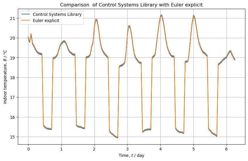
Figure 4. Time variation of indoor temperature obtained with Control Systems Library and for-loop Euler.
# Print the comparison of durations
print(f"Duration for Control Systems Library: {duration_1:.2f} seconds")
print(f"Duration for Euler explict:           {duration_2:.2f} seconds")
Duration for Control Systems Library: 2.36 seconds
Duration for Euler explict:           15.80 seconds
Controller influence on time step#
Simulate the system without controller (i.e., in free floating) and with controller.
Note that the time step for Euler explicit method depends on:
Gain
TC['G']['q11'] = Kpof the P-controller:if \(K_p \rightarrow \infty\), then the controller is perfect and the time step needs to be small;
if \(K_p \rightarrow 0\), then, the controller is ineffective and the building is in free-running.
Capacities considered into the model:
if the capacities of the air \(C_a =\)
C['Air']and of the glass \(C_g =\)C['Glass']are considered, then the time step is small;if the capacities of the air,
TC['C']['θ6'], and of the glass,TC['C']['θ6'], are zero, then the time step is large (and the order of the state-space model is reduced).
The controller models an HVAC system able to heat (when \(q_{HVAC} > 0\)) and to cool (when \(q_{HVAC} < 0\)) when \(K_p \approx 10^3 \ \mathrm{W/K}\). Change \(K_p \approx 10^2 \ \mathrm{W/K}\) and \(K_p \approx 10^4 \ \mathrm{W/K}.\)
References#
C. Ghiaus (2013). Causality issue in the heat balance method for calculating the design heating and cooling loads, Energy 50: 292-301, , open access preprint: HAL-03605823
C. Ghiaus (2021). Dynamic Models for Energy Control of Smart Homes, in S. Ploix M. Amayri, N. Bouguila (eds.) Towards Energy Smart Homes, Online ISBN: 978-3-030-76477-7, Print ISBN: 978-3-030-76476-0, Springer, pp. 163-198, open access preprint: HAL 03578578
J.A. Duffie, W. A. Beckman, N. Blair (2020). Solar Engineering of Thermal Processes, 5th ed. John Wiley & Sons, Inc. ISBN 9781119540281
Réglementation Thermique 2005. Méthode de calcul Th-CE.. Annexe à l’arrêté du 19 juillet 2006
H. Recknagel, E. Sprenger, E.-R. Schramek (2013) Génie climatique, 5e edition, Dunod, Paris. ISBN 978-2-10-070451-4
J.R. Howell et al. (2021). Thermal Radiation Heat Transfer 7th edition, ISBN 978-0-367-34707-0, A Catalogue of Configuration Factors
J. Widén, J. Munkhammar (2019). Solar Radiation Theory, Uppsala University