Nonlinear controller

This notebook, which uses dm4bem module, shows how to change the control input during the numerical integration in order to implement complex control algorithms. The procedure presented in Inputs and simulation is used with the difference that nonlinear control algorithms are implemented in the time-integration loop.

import numpy as np
import pandas as pd
import matplotlib.pyplot as plt

import dm4bem

def control_for(controller, period, dt=30, nonlinear_controller=True):
    # Obtain state-space representation
    # =================================
    # Disassembled thermal circuits
    folder_path = './pd/bldg'
    TCd = dm4bem.bldg2TCd(folder_path,
                          TC_auto_number=True)

    # Assembled thermal circuit
    ass_lists = pd.read_csv(folder_path + '/assembly_lists.csv')
    ass_matrix = dm4bem.assemble_lists2matrix(ass_lists)
    TC = dm4bem.assemble_TCd_matrix(TCd, ass_matrix)

    # TC['G']['c3_q0'] = 1e3  # Kp, controler gain
    # TC['C']['c2_θ0'] = 0    # indoor air heat capacity
    # TC['C']['c1_θ0'] = 0    # glass (window) heat capacit

    # State-space
    [As, Bs, Cs, Ds, us] = dm4bem.tc2ss(TC)

    # Eigenvaleus analysis
    # ====================
    λ = np.linalg.eig(As)[0]    # eigenvalues of matrix As

    dt_max = 2 * min(-1. / λ)    # max time step for Euler explicit stability
    dt_max = dm4bem.round_time(dt_max)
    # dm4bem.print_rounded_time('dt_max', dt)

    # Simulation with weather data
    # ============================
    # Start / end time
    start_date = period[0]
    end_date = period[1]

    start_date = '2000-' + start_date
    end_date = '2000-' + end_date

    # Weather
    filename = '../weather_data/FRA_Lyon.074810_IWEC.epw'
    [data, meta] = dm4bem.read_epw(filename, coerce_year=None)
    weather = data[["temp_air", "dir_n_rad", "dif_h_rad"]]
    del data
    weather.index = weather.index.map(lambda t: t.replace(year=2000))
    weather = weather.loc[start_date:end_date]

    # Temperature sources
    To = weather['temp_air']

    Ti_day, Ti_night = 20, 16
    Ti_sp = pd.Series(20, index=To.index)
    Ti_sp = pd.Series(
        [Ti_day if 6 <= hour <= 22 else Ti_night for hour in To.index.hour],
        index=To.index)

    # Flow-rate sources
    # total solar irradiance
    wall_out = pd.read_csv('pd/bldg/walls_out.csv')
    w0 = wall_out[wall_out['ID'] == 'w0']

    surface_orientation = {'slope': w0['β'].values[0],
                           'azimuth': w0['γ'].values[0],
                           'latitude': 45}

    rad_surf = dm4bem.sol_rad_tilt_surf(
        weather, surface_orientation, w0['albedo'].values[0])

    Etot = rad_surf.sum(axis=1)

    # Window glass properties
    α_gSW = 0.38    # short wave absortivity: reflective blue glass
    τ_gSW = 0.30    # short wave transmitance: reflective blue glass
    S_g = 9         # m2, surface area of glass

    # Flow-rate sources
    # solar radiation
    Φo = w0['α1'].values[0] * w0['Area'].values[0] * Etot
    Φi = τ_gSW * w0['α0'].values[0] * S_g * Etot
    Φa = α_gSW * S_g * Etot

    # auxiliary (internal) sources
    Qa = pd.Series(0, index=To.index)

    # Input data set
    input_data_set = pd.DataFrame({'To': To, 'Ti_sp': Ti_sp,
                                   'Φo': Φo, 'Φi': Φi, 'Qa': Qa, 'Φa': Φa,
                                   'Etot': Etot})

    # Time integration
    # ----------------
    # Resample hourly data to time step dt
    input_data_set = input_data_set.resample(
        str(dt) + 'S').interpolate(method='linear')

    # Get input from input_data_set
    u = dm4bem.inputs_in_time(us, input_data_set)

    # initial conditions
    θ0 = 20.0                   # initial temperatures
    θ_exp = pd.DataFrame(index=u.index)
    θ_exp[As.columns] = θ0      # Fill θ with initial valeus θ0

    # time integration
    I = np.eye(As.shape[0])     # identity matrix

    for k in range(1, u.shape[0] - 1):
        if nonlinear_controller:
            exec(controller)

        θ_exp.iloc[k + 1] = (I + dt * As)\
            @ θ_exp.iloc[k] + dt * Bs @ u.iloc[k]

    # outputs
    y = (Cs @ θ_exp.T + Ds @  u.T).T

    Kp = TC['G']['c3_q0']     # W/K, controller gain
    S = 3 * 3                 # m², surface area of the toy house

    # q_HVAC / [W/m²]
    if nonlinear_controller:
        q_HVAC = u['c2_θ0']
    else:
        q_HVAC = Kp * (u['c3_q0'] - y['c2_θ0']) / S  # W/m²

    # plot
    data = pd.DataFrame({'To': input_data_set['To'],
                         'θi': y['c2_θ0'],
                         'Etot': input_data_set['Etot'],
                         'q_HVAC': q_HVAC})

    fig, axs = plt.subplots(2, 1, sharex=True)
    data[['To', 'θi']].plot(ax=axs[0],
                            xticks=[],
                            ylabel='Temperature, $θ$ / °C')
    axs[0].legend(['$θ_{outdoor}$', '$θ_{indoor}$'],
                  loc='upper right')
    axs[0].grid(True)

    data[['Etot', 'q_HVAC']].plot(ax=axs[1],
                                  ylabel='Heat rate, $q$ / (W·m⁻²)')
    axs[1].set(xlabel='Time')
    axs[1].legend(['$E_{total}$', '$q_{HVAC}$'],
                  loc='upper right')
    axs[1].grid(True)
    plt.show()

Model

Figure 1. Assembled circuit.

In this example, we will consider that the controller is not modeled by the conductance \(G_0\) and the temperature source \(T_{i,sp}\) of circuit TC3:c3 but, instead, by the heatflow rate \(\dot{Q}_a\), which is added to the indoor air in node \(\theta_0\) of circuit TC2:c2 (Figure 1). Therefore, in TC3:c3 the conductance \(G_0 \rightarrow 0\) and

\[\dot{Q}_a \equiv u_{c2\_θ0} = K_p (T_{i,sp} - \theta_{c2\_θ0})\]

where:

• \(\dot{Q}_a\) - auxiliary heat in node θ0 of circuit c2, W;

• \(u_{c2\_θ0}\) - input of type flow rate source in node θ0 of circuit c2, W;

• \(K_p\) - static gain of the proportional controller, W/°C;

• \(T_{i,sp}\) - indoor temperature setpoint, °C;

• \(\theta_{c2\_θ0}\) - indoor temperature, which is the temperature node θ0 of circuit c2, °C.

Free running

The model can be simulated in free-runinng when there is no nonlinear controller (i.e., \(\dot{Q}_a = 0\)).

start_date = '02-01 12:00:00'
end_date = '02-03 18:00:00'
period = [start_date, end_date]

control_for("free running", period, dt=30,
            nonlinear_controller=False)

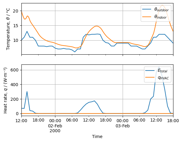
Figure 2. Free-running (i.e., no controller).

Heating

In heating, the auxiliary heat flow \(\dot{Q}_a \equiv u_{c2\_θ0}\) is zero if the indoor air temperature \(\theta_{c2\_θ0}\) is higher than its setpoint \(T_{i,sp}\). Otherwise, the input is

\[u_{c2\_θ0} = K_p (T_{i,sp} - \theta_{c2\_θ0})\]

if \(u_{c2\_θ0} > 0\).

heating = """
Tisp = 20   # indoor setpoint temperature, °C
Kpp = 1e3   # controller gain

if Tisp < θ_exp.iloc[k - 1]['c2_θ0']:
    u.iloc[k]['c2_θ0'] = 0
else:
    u.iloc[k]['c2_θ0'] = Kpp * (Tisp - θ_exp.iloc[k - 1]['c2_θ0'])
"""

control_for(heating, period)

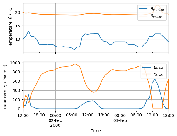
Figure 3. Heating.

Cooling

In cooling, the auxiliary heat flow \(\dot{Q}_a \equiv u_{c2\_θ0}\) is zero if the indoor air temperature \(\theta_{c2\_θ0}\) is lower than its setpoint \(T_{i,sp}\). Otherwise, the input is

\[u_{c2\_θ0} = K_p (T_{i,sp} - \theta_{c2\_θ0})\]

cooling = """
Tisp = 20   # indoor setpoint temperature, °C
Δθ = 5      # temperature deadband, °C
Kpp = 1e2   # controller gain

if θ_exp.iloc[k - 1]['c2_θ0'] < Tisp + Δθ :
    u.iloc[k]['c2_θ0'] = 0
else:
    u.iloc[k]['c2_θ0'] = Kpp * (Tisp - θ_exp.iloc[k - 1]['c2_θ0'])
"""
period = ['07-01 12:00:00', '07-03 12:00:00']
control_for(cooling, period)

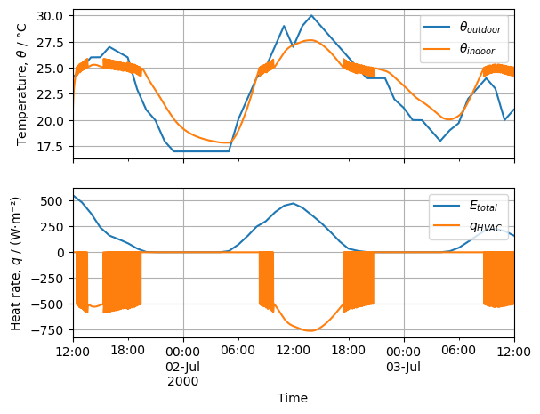
Figure 4. Cooling.

Heating and cooling with deadband

During mid-season, heating and cooling may be required. In this case a deadband controller is preferred to a perfect controller (see Inputs and simulation). In deadband controller, the auxiliary heat flow \(\dot{Q}_a \equiv u_{c2\_θ0}\) is zero if the indoor air temperature \(\theta_{c2\_θ0}\) is higher than its setpoint \(T_{i,sp}\) but lower than the setpoint plus the deadband \(\Delta \theta\). Otherwise, the input is

\[u_{c2\_θ0} = K_p (T_{i,sp} - \theta_{c2\_θ0})\]

heat_cool = """
Tisp = 20   # indoor setpoint temperature, °C
Δθ = 5      # temperature deadband, °C
Kpp = 3e2   # controller gain

if Tisp < θ_exp.iloc[k - 1]['c2_θ0'] < Tisp + Δθ:
    u.iloc[k]['c2_θ0'] = 0
else:
    u.iloc[k]['c2_θ0'] = Kpp * (Tisp - θ_exp.iloc[k - 1]['c2_θ0'])
"""
period = ['05-01 12:00:00', '05-03 12:00:00']
control_for(heat_cool, period)

Figure 5. Heating and cooling with deadband.

Solar protection

The cooling load can be reduced by solar protection. In our example, let’s assume that if the indoor temperature is higher than its setpoint, exterior shutters are closed. To model this, the flow rate \(\Phi_i\) in node \(\theta_4\) of thermal circuit walls_out: ow0, i.e. \(u_{ow0\_θ4}\) (Figure 1), is reduced at 10 % of its value.

solar_protection = """
Tisp = 20   # indoor setpoint temperature, °C
Δθ = 1      # temperature deadband, °C
Kpp = 3e2   # controller gain

if θ_exp.iloc[k - 1]['c2_θ0'] < Tisp + Δθ:
    u.iloc[k]['c2_θ0'] = 0
else:
    u.iloc[k]['c2_θ0'] = Kpp * (Tisp - θ_exp.iloc[k - 1]['c2_θ0'])
    u.iloc[k]['c2_θ0'] = min(u.iloc[k]['c2_θ0'], 0)
    u.iloc[k]['ow0_θ4'] *= 0.1
"""

period = ['05-01 12:00:00', '05-03 12:00:00']
control_for(solar_protection, period)

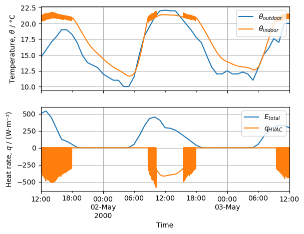
Figure 6. Cooling load is reduced by solar protection.

Passive cooling

In mid-season, the building may be cooled by using passive cooling techniques, such as solar protection with window shutters and free cooling.

Free-cooling is modeled by increasing the air changes per hour (ACH). In our example, ventilation rate is increased from 1 ACH to 10 ACH and the cooling is turned off, u.iloc[k]['c2_θ0'] = 0.

The thermal conductance for free-cooling by ventilation is

\[G_{free} = \dot{m}_a c_a = \rho_a c_a \dot{V}_a\]

where:

• \(\dot{m}_a\) is the mass flow rate of air, kg/s;

• \(\dot{V}_a\) - volumetric flow rate, m³/s;

• \(c_a\) - specific heat capacity of the air, J/kg·K;

• \(\rho_a\) - density of air, kg/m³.

The volumetric flow rate of the air, in m³/s, is:

\[\dot{V}_a = \frac{\mathrm{ACH}}{3600} V_a\]

where:

• \(\mathrm{ACH}\) (air changes per hour) is the air infiltration rate, 1/h;

• \(3600\) - number of seconds in one hour, s/h;

• \(V_a\) - volume of the air in the thermal zone, m³.

The net flow rate that the building receives by advection, i.e., introducing outdoor air at temperature \(T_o\) and extracting indoor air at temperature \(\theta_i\) by ventilation, is:

\[q_{free} = G_{free} (T_o - \theta_i)\]

where:

• \(T_o\) - outdoor air temperature, °C, is u['ow0_q0'] (Figure 1);

• \(\theta_i\) - indoor air temperature, °C, is θ_exp['c2_θ0'].

Modifying the conductance for advection, \(G_0\) in thermal circuit TC2: c2 (Figure 1), implies recalculating the state-space model. As an altenative, we can consider that the flow rate

\[q_{free} = G_{free} (T_o - \theta_i)\]

implemented as q_free = G_free * (u['ow0_q0'] - θ_exp['c2_θ0']), is added to \(Q_a\), which is input u['c2_θ0'] (Figure 1).

passive_cooling = """
Tisp = 20.0                 # indoor setpoint temperature, °C
Δθ = 1.0                    # temperature deadband, °C
Kpp = 3e2                   # controller gain

# ventilation flow rate
l = 3.0                     # m length of the cubic room
Va = l**3                   # m³, volume of air
ACH = 10.0                  # 1/h, air changes per hour
Va_dot = ACH / 3600 * Va    # m³/s, air infiltration
ρ = 1.2                     # kg/m³
c = 1000.0                  # J/(kg·K)
G_free = ρ * c * Va_dot
q_free = G_free * (u.iloc[k - 1]['ow0_q0'] - θ_exp.iloc[k - 1]['c2_θ0'])

if θ_exp.iloc[k - 1]['c2_θ0'] < Tisp + Δθ:
    u.iloc[k]['c2_θ0'] = 0
else:
    u.iloc[k]['c2_θ0'] = 0
    if u.iloc[k - 1]['ow0_q0'] < Tisp:
        u.iloc[k]['c2_θ0'] = q_free
    u.iloc[k]['ow0_θ4'] *= 0.1
"""

period = ['05-01 12:00:00', '05-03 12:00:00']
control_for(passive_cooling, period)

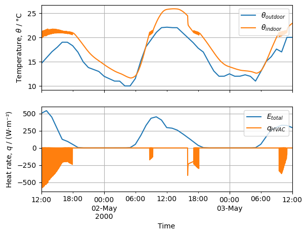
Figure 7. Solar protection and free-cooling.