Steady-state and step response#
![]()
Steady-state analysis focuses on the behavior of a system after transients have settled, specifically when the system reaches a stable equilibrium at a constant input.
Step response analyses system’s dynamic response to a sudden change in input (i.e., to a step input). Step response is concerned with transient behavior, such as how the system responds immediately after the input change and how it eventually settles into a new steady-state.
Objectives:
Find the steady-state values for thermal circuit and state-space.
Estimate the time step and the settling time from eigenvalue analysis.
Simulate the step response.
Compare the steady-state results with step response after settling time.

Figure 1. Thermal circuit for the cubic building.
import numpy as np
import pandas as pd
import matplotlib.pyplot as plt

import dm4bem
The following assumptions are done:
The indoor air temperature is controlled or not (i.e., the building is in free running).
The heat capacity of air and of glass is neglected or not.
The time step is calculated from the eigenvalues or it is imposed at a value designated as \(\Delta t\).
controller = False
neglect_air_glass_capacity = False
imposed_time_step = False
Δt = 498    # s, imposed time step
The thermal circuit was described in the section on modelling (Figure 1). It is given by a thermal circuit imported from the file ./toy_model/TC.csv.
A thermal ciruit file contains the incidence matrix \(A\), the diagonals of matrices \(G\) and \(C\), and the vectors \(b\), \(f\), and \(y\) (see example below). If there is no value in a cell, it is considered 0.
print('Matrices and vectors for thermal circuit from Figure 1')
df = pd.read_csv('./toy_model/TC_0.csv')
df.style.apply(lambda x: ['background-color: yellow'
                          if x.name in df.index[-3:] or c in df.columns[-2:]
                          else '' for c in df.columns], axis=1)
Matrices and vectors for thermal circuit from Figure 1
| A | θ0 | θ1 | θ2 | θ3 | θ4 | θ5 | θ6 | θ7 | G | b | |
|---|---|---|---|---|---|---|---|---|---|---|---|
| 0 | q0 | 1 | 0.000000 | 0 | 0 | 0 | 0 | 0 | 0 | 1125.000000 | To |
| 1 | q1 | -1 | 1.000000 | 0 | 0 | 0 | 0 | 0 | 0 | 630.000000 | 0 |
| 2 | q2 | 0 | -1.000000 | 1 | 0 | 0 | 0 | 0 | 0 | 630.000000 | 0 |
| 3 | q3 | 0 | 0.000000 | -1 | 1 | 0 | 0 | 0 | 0 | 30.375000 | 0 |
| 4 | q4 | 0 | 0.000000 | 0 | -1 | 1 | 0 | 0 | 0 | 30.375000 | 0 |
| 5 | q5 | 0 | 0.000000 | 0 | 0 | -1 | 1 | 0 | 0 | 44.786824 | 0 |
| 6 | q6 | 0 | 0.000000 | 0 | 0 | -1 | 0 | 1 | 0 | 360.000000 | 0 |
| 7 | q7 | 0 | 0.000000 | 0 | 0 | 0 | -1 | 1 | 0 | 72.000000 | 0 |
| 8 | q8 | 0 | 0.000000 | 0 | 0 | 0 | 0 | 0 | 1 | 165.789474 | To |
| 9 | q9 | 0 | 0.000000 | 0 | 0 | 0 | 1 | 0 | -1 | 630.000000 | 0 |
| 10 | q10 | 0 | 0.000000 | 0 | 0 | 0 | 0 | 1 | 0 | 9.000000 | To |
| 11 | q11 | 0 | 0.000000 | 0 | 0 | 0 | 0 | 1 | 0 | 0.000000 | Ti_sp |
| 12 | C | 0 | 18216000.000000 | 0 | 239580 | 0 | 0 | 32400 | 1.089E+06 | nan | nan |
| 13 | f | Φo | 0.000000 | 0 | 0 | Φi | 0 | Qa | Φa | nan | nan |
| 14 | y | 0 | 0.000000 | 0 | 0 | 0 | 0 | 1 | 0 | nan | nan |
In the thermal circuit ./toy_model/TC.csv, the controller is off, i.e., the gain of the proportional controller is 0, \(K_p = G_{11} = 0\); the building is in free-floating. The controller may be turned on by setting \(K_p = G_{11} \rightarrow \infty\).
# MODEL
# =====
# Thermal circuit
TC = dm4bem.file2TC('./toy_model/TC.csv', name='', auto_number=False)

# by default TC['G']['q11'] = 0, i.e. Kp -> 0, no controller (free-floating)
if controller:
    TC['G']['q11'] = 1e3        # Kp -> ∞, almost perfect controller

if neglect_air_glass_capacity:
    TC['C']['θ6'] = TC['C']['θ7'] = 0
    # or
    TC['C'].update({'θ6': 0, 'θ7': 0})
Thermal circuit is transformed in state-space representation.
# State-space
[As, Bs, Cs, Ds, us] = dm4bem.tc2ss(TC)
Steady-state analysis#
Steady-state means that the temperatures do not vary in time. In the system of differential-algebraic equations (DAE):
the term \(\dot \theta = 0\), or in the state-space representation,
the term \(\dot \theta_s = 0\).
In steady-state, the model can be checked if it is incorrect. Let’s consider that:
the controller is not active, \(K_p \rightarrow 0\),
the outdoor temperature is \(T_o = 10 \, \mathrm{^\circ C}\),
the indoor temperature setpoint is \(T_{i,sp} = 20 \, \mathrm{^\circ C}\),
all flow rate sources are zero.
bss = np.zeros(12)        # temperature sources b for steady state
bss[[0, 8, 10]] = 10      # outdoor temperature
bss[[11]] = 20            # indoor set-point temperature

fss = np.zeros(8)         # flow-rate sources f for steady state
Note: Steady-state analysis is a test of falsification (refutability) of the model, not a verification and validation. If the model does not pass the steady-state test, it means that it is wrong. If the model passes the steady-state test, it does not mean that it is correct. For this example, the values of the capacities in matrix \(C\) or of the conductances in matrix \(G\) can be wrong, even when the steady-state test is passed.
Steady-state from differential algebraic equations (DAE)#
The temperature values in steady-state are obtained from the system of DAE by considering that \(C \dot{\theta} = 0\):
For the conditions mentioned above, in steady-state, all temperatures \(\theta_0 ... \theta_7,\) including the indoor air temperature \(\theta_6,\) are equal to \(T_o = 10 \, \mathrm{^\circ C}\) (Figure 1).
A = TC['A']
G = TC['G']
diag_G = pd.DataFrame(np.diag(G), index=G.index, columns=G.index)

θss = np.linalg.inv(A.T @ diag_G @ A) @ (A.T @ diag_G @ bss + fss)
print(f'θss = {np.around(θss, 2)} °C')
θss = [10. 10. 10. 10. 10. 10. 10. 10.] °C
If the sum of the auxiliary heat sources in the room, \(\dot Q_a = f_6\), is not zero, the temperature in the room \(\theta_6\) has the highest value and the temperature of the outdoor surface of the wall \(\theta_0\) is almost equal to the outdoor temperature, \(T_o = b_0\).
bss = np.zeros(12)        # temperature sources b for steady state

fss = np.zeros(8)         # flow-rate sources f for steady state
fss[[6]] = 1000

θssQ = np.linalg.inv(A.T @ diag_G @ A) @ (A.T @ diag_G @ bss + fss)
print(f'θssQ = {np.around(θssQ, 2)} °C')
θssQ = [ 0.14 0.39 0.65 5.88 11.12 5.57 12.26 4.41] °C
Steady-state from state-space representation#
The input vector \(u\) of the state-space representation is obtained by stacking the vectors \(b_T\) and \(f_Q\):
where:
\(b_T\) is a vector of the nonzero elements of vector \(b\) of temperature sources. For the circuit presented in Figure 1, \(b_T = [T_o, T_o, T_o, T_{i,sp}]^T\) corresponding to branches 0, 8, 10 and 11, where:
\(T_o\) - outdoor temperature, °C;
\(T_{i,sp}\) - set-point temperaure for the indoor air, °C.
\(f_Q\) - vector of nonzero elements of vector \(f\) of flow sources. For the circuit presented in Figure 1, \(f_Q = [\Phi_o, \Phi_i, \dot{Q}_a, \Phi_a]^T\), corresponding to nodes 0, 4, 6, and 7, where:
\(\Phi_o\) - solar radiation absorbed by the outdoor surface of the wall, W;
\(\Phi_i\) - solar radiation absorbed by the indoor surface of the wall, W;
\(\dot{Q}_a\) - auxiliary heat gains (i.e., occupants, electrical devices, etc.), W;
\(\Phi_a\) - solar radiation absorbed by the glass, W.
Note: Zero in vectors \(b\) and \(f\) indicates that there is no source on the branch or in the node, respectively. However, a source can have the value zero.
bT = np.array([10, 10, 10, 20])     # [To, To, To, Tisp]
fQ = np.array([0, 0, 0, 0])         # [Φo, Φi, Qa, Φa]
uss = np.hstack([bT, fQ])           # input vector for state space
print(f'uss = {uss}')
uss = [10 10 10 20 0 0 0 0]
The steady-state value of the output of the state-space representation is obtained when \(\dot \theta_{C} = 0\):
inv_As = pd.DataFrame(np.linalg.inv(As),
                      columns=As.index, index=As.index)
yss = (-Cs @ inv_As @ Bs + Ds) @ uss

yss = float(yss.values[0])
print(f'yss = {yss:.2f} °C')
yss = 10.00 °C
The error between the steady-state values obtained from the system of DAE, \(\theta_6\), and the output of the state-space representation, \(y_{ss}\),
is practically zero; the slight difference is due to numerical errors.
print(f'Error between DAE and state-space: {abs(θss[6] - yss):.2e} °C')
Error between DAE and state-space: 8.88e-15 °C
Likewise, the steady-state of the output of the state-space representation for input \(\dot Q_a\) is obtained from
bT = np.array([0, 0, 0, 0])         # [To, To, To, Tisp]
fQ = np.array([0, 0, 1000, 0])      # [Φo, Φi, Qa, Φa]
uss = np.hstack([bT, fQ])

inv_As = pd.DataFrame(np.linalg.inv(As),
                      columns=As.index, index=As.index)
yssQ = (-Cs @ inv_As @ Bs + Ds) @ uss

yssQ = float(yssQ.values[0])
print(f'yssQ = {yssQ:.2f} °C')
yssQ = 12.26 °C
The steady-state values obtained from DAE and state-space representation are pratically equal.
print(f'Error between DAE and state-space: {abs(θssQ[6] - yssQ):.2e} °C')
Error between DAE and state-space: 7.11e-15 °C
Eigenvalues analysis#
Let’s consider the eigenvalues \(\lambda\) of the state matrix \(A_s\).
# Eigenvalues analysis
λ = np.linalg.eig(As)[0]        # eigenvalues of matrix As
Time step#
The condition for numerical stability of Euler explicit integration method is
i.e., in the complex plane, \(\lambda_i \Delta t\) is inside a circle of radius 1 centered in \((-1 + 0j) \in \mathbb{C}\), where:
\(\lambda_i\) are the eigenvalues of matrix \(A_s\),
\(\Delta t\) - time step,
\(j = \sqrt {-1}\) - imaginary unit.
For real negative eigenvalues \(\left \{ \lambda_i \in \mathbb{R} \;| \; \lambda_i <0 \right \}\), which is the case of thermal networks, the above condition becomes:
or
where \(T_i\) are the time constants, \(T_i = - 1 / \lambda_i\). Let’s chose a time step \(dt\) smaller than \(\Delta t_{max} = 2 \min (-1 / \lambda_i) \), floor rounded to:
1 s, 10 s,
60 s (1 min), 300 s (5 min), 600 s (10 min), 1800 s (30 min),
36000 s (1 h), 7200 s (2 h), 14400 s (4 h), 21600 s (6 h).
# time step
Δtmax = 2 * min(-1. / λ)    # max time step for stability of Euler explicit
dm4bem.print_rounded_time('Δtmax', Δtmax)

if imposed_time_step:
    dt = Δt
else:
    dt = dm4bem.round_time(Δtmax)

dm4bem.print_rounded_time('dt', dt)
print(f"dt = {dt:.0f} s")
Δtmax = 498 s = 8.3 min
dt = 300 s = 5.0 min
dt = 300 s
if dt < 10:
    raise ValueError("Time step is too small. Stopping the script.")
Settling time and duration#
The settling time at less than 5 % (i.e., \(e^{-3}\)) of the final value is roughly 3 times the largest time constant (and less than 1 % (i.e., \(e^{-5}\)) of the final value for 5 times the largest time constant).
# settling time
t_settle = 4 * max(-1 / λ)
dm4bem.print_rounded_time('t_settle', t_settle)
t_settle = 176132 s = 48.9 h
The duration of the simulation needs to be larger than the estimated settling time. This requires a corresponding number of time steps in the time vector.
# duration: next multiple of 3600 s that is larger than t_settle
duration = np.ceil(t_settle / 3600) * 3600
dm4bem.print_rounded_time('duration', duration)
duration = 176400 s = 49.0 h
Step response to outdoor temperature#
Input vector#
In dynamic simulation, the inputs are time series, e.g., the oudoor temperature will have \(n\) values \(T_o = [T_{o(0)}, T_{o(1)}, ..., T_{o(n-1)}]\) at discrete time \(t = [t_0, t_1, ... , t_{n-1}]\).
The input vector \(u\) of the state-space representation is obtained by stacking the vectors \(b_T\) and \(f_Q\) of the system of Differential Algebraic Equations:
where:
vector \(b_T\) consists of the nonzero elements of vector \(b\) of temperature sources; for the circuit presented in Figure 1,
and
corresponding to branches 0, 8, 10 and 11;
vector \(f_Q\) is the nonzero elements of vector \(f\) of flow sources; for the circuit presented in Figure 1,
and
corresponding to nodes 0, 4, 6, and 7.
For the thermal circuit shown in Figure 1, the time series of the input vector, \(u = [u_0, u_1, ... , u_{n-1}]^T\), is:
where:
\(T_o = [T_{o(0)}, T_{o(1)}, ..., T_{o(n-1)}]\) is the time series of the oudoor temperature at discrete time \(t = [t_0, t_1, ... , t_{n-1}]\).
\(T_{i, sp} = [T_{{i, sp}(0)}, T_{{i, sp}(1)}, ..., T_{{i, sp}(n-1)}]\) is the time series of the setpoint indoor temperature at discrete time \(t = [t_0, t_1, ... , t_{n-1}]\).
\(\Phi_o = [\Phi_{o(0)}, \Phi_{o(1)}, ..., \Phi_{o(n-1)}]\) is the time series of the solar radiation absorbed by the outdoor surface of the wall at discrete time \(t = [t_0, t_1, ... , t_{n-1}]\).
\(\Phi_i = [\Phi_{i(0)}, \Phi_{i(1)}, ..., \Phi_{i(n-1)}]\) is the time series of the solar radiation absorbed by the indoor surface of the wall at discrete time \(t = [t_0, t_1, ... , t_{n-1}]\).
\(\dot{Q}_a = [\dot{Q}_{a(0)}, \dot{Q}_{a(1)}, ..., \dot{Q}_{a(n-1)}]\) is the time series of the auxiliary heat gains (i.e., occupants, electrical devices, etc.) at discrete time \(t = [t_0, t_1, ... , t_{n-1}]\).
\(\Phi_a = [\Phi_{a(0)}, \Phi_{a(1)}, ..., \Phi_{a(n-1)}]\) is the time series of the solar radiation absorbed by the glass at discrete time \(t = [t_0, t_1, ... , t_{n-1}]\).
Note: In Pandas time series, time is an index. Therefore, Pandas representation of vector of inputs \(u\) in time is the transpose of the matrix presented above.
Let’s consider a step response in the conditions used for steady-state analysis, i.e., \(T_o = 10 \, \mathrm{^\circ C}\), \(T_{i,sp} = 20 \, \mathrm{^\circ C}\), and all the flow sources zero (including the HVAC system).
# Create input_data_set
# ---------------------
# time vector
n = int(np.floor(duration / dt))    # number of time steps

# DateTimeIndex starting at "00:00:00" with a time step of dt
time = pd.date_range(start="2000-01-01 00:00:00",
                           periods=n, freq=f"{int(dt)}s")

To = 10 * np.ones(n)        # outdoor temperature
Ti_sp = 20 * np.ones(n)     # indoor temperature set point
Φa = 0 * np.ones(n)         # solar radiation absorbed by the glass
Qa = Φo = Φi = Φa           # auxiliary heat sources and solar radiation

data = {'To': To, 'Ti_sp': Ti_sp, 'Φo': Φo, 'Φi': Φi, 'Qa': Qa, 'Φa': Φa}
input_data_set = pd.DataFrame(data, index=time)

# inputs in time from input_data_set
u = dm4bem.inputs_in_time(us, input_data_set)
Time integration#
The state-space model
is integrated in time by using Euler forward (or explicit) method for numerical integration:
and Euler backward (or implicit) method for numerical integration:
where \(k = 0, ... , n - 1\).
# Initial conditions
θ_exp = pd.DataFrame(index=u.index)     # empty df with index for explicit Euler
θ_imp = pd.DataFrame(index=u.index)     # empty df with index for implicit Euler

θ0 = 0.0                    # initial temperatures
θ_exp[As.columns] = θ0      # fill θ for Euler explicit with initial values θ0
θ_imp[As.columns] = θ0      # fill θ for Euler implicit with initial values θ0

I = np.eye(As.shape[0])     # identity matrix
for k in range(u.shape[0] - 1):
    θ_exp.iloc[k + 1] = (I + dt * As)\
        @ θ_exp.iloc[k] + dt * Bs @ u.iloc[k]
    θ_imp.iloc[k + 1] = np.linalg.inv(I - dt * As)\
        @ (θ_imp.iloc[k] + dt * Bs @ u.iloc[k])
Then, we obtain the outputs
for explicit and for implicit Euler methods, respectively.
# outputs
y_exp = (Cs @ θ_exp.T + Ds @  u.T).T
y_imp = (Cs @ θ_imp.T + Ds @  u.T).T
# plot results
y = pd.concat([y_exp, y_imp], axis=1, keys=['Explicit', 'Implicit'])
# Flatten the two-level column labels into a single level
y.columns = y.columns.get_level_values(0)

ax = y.plot()
ax.set_xlabel('Time')
ax.set_ylabel('Indoor temperature, $\\theta_i$ / °C')
ax.set_title(f'Time step: $dt$ = {dt:.0f} s; $dt_{{max}}$ = {Δtmax:.0f} s')
plt.show()
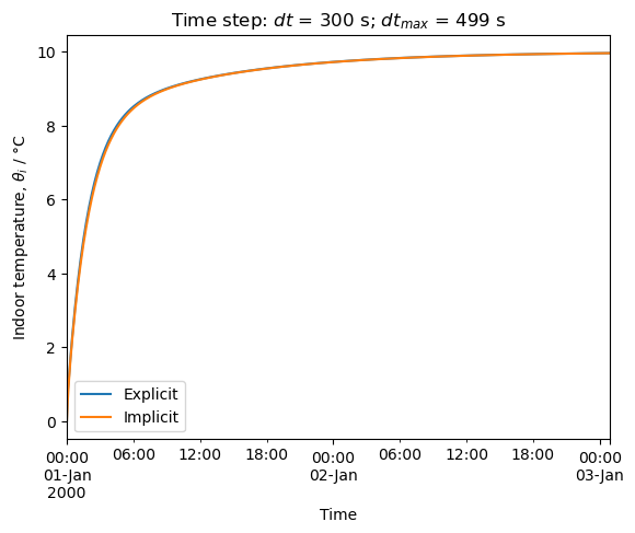
The results of explicit and implicit Euler integration are practically identical if \(dt < dt_{max}\). If \(dt > dt_{max}\), Euler explicit method of integration is numerically unstable.
The value the indoor temperature obtained after the settling time is almost equal to the value obtained in steady-state.
print('Steady-state indoor temperature obtained with:')
print(f'- DAE model: {float(θss[6]):.4f} °C')
print(f'- state-space model: {float(yss):.4f} °C')
print(f'- steady-state response to step input: \
{y_exp["θ6"].tail(1).values[0]:.4f} °C')
Steady-state indoor temperature obtained with:
- DAE model: 10.0000 °C
- state-space model: 10.0000 °C
- steady-state response to step input: 9.9645 °C
Step response to internal load#
Let’s consider that the temperature sources are zero and that the flow-rate sources are zero, with the exception of the auxiliary heat gains, \(\dot Q_a\).
# Create input_data_set
# ---------------------
# time vector
n = int(np.floor(duration / dt))    # number of time steps

# Create a DateTimeIndex starting at "00:00:00" with a time step of dt
time = pd.date_range(start="2000-01-01 00:00:00",
                           periods=n, freq=f"{int(dt)}s")
# Create input_data_set
To = 0 * np.ones(n)         # outdoor temperature
Ti_sp =  20 * np.ones(n)     # indoor temperature set point
Φa = 0 * np.ones(n)         # solar radiation absorbed by the glass
Φo = Φi = Φa                # solar radiation
Qa = 1000 * np.ones(n)      # auxiliary heat sources
data = {'To': To, 'Ti_sp': Ti_sp, 'Φo': Φo, 'Φi': Φi, 'Qa': Qa, 'Φa': Φa}
input_data_set = pd.DataFrame(data, index=time)

# Get inputs in time from input_data_set
u = dm4bem.inputs_in_time(us, input_data_set)
# Initial conditions
θ_exp[As.columns] = θ0      # fill θ for Euler explicit with initial values θ0
θ_imp[As.columns] = θ0      # fill θ for Euler implicit with initial values θ0

I = np.eye(As.shape[0])     # identity matrix
for k in range(u.shape[0] - 1):
    θ_exp.iloc[k + 1] = (I + dt * As)\
        @ θ_exp.iloc[k] + dt * Bs @ u.iloc[k]
    θ_imp.iloc[k + 1] = np.linalg.inv(I - dt * As)\
        @ (θ_imp.iloc[k] + dt * Bs @ u.iloc[k])
# outputs
y_exp = (Cs @ θ_exp.T + Ds @  u.T).T
y_imp = (Cs @ θ_imp.T + Ds @  u.T).T
# plot results
y = pd.concat([y_exp, y_imp], axis=1, keys=['Explicit', 'Implicit'])
# Flatten the two-level column labels into a single level
y.columns = y.columns.get_level_values(0)
ax = y.plot()
ax.set_xlabel('Time')
ax.set_ylabel('Indoor temperature, $\\theta_i$ / °C')
ax.set_title(f'Time step: $dt$ = {dt:.0f} s; $dt_{{max}}$ = {Δtmax:.0f} s')
plt.show()
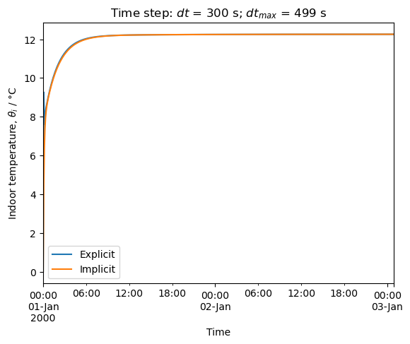
print('Steady-state indoor temperature obtained with:')
print(f'- DAE model: {float(θssQ[6]):.4f} °C')
print(f'- state-space model: {float(yssQ):.4f} °C')
print(f'- steady-state response to step input: \
{y_exp["θ6"].tail(1).values[0]:.4f} °C')
Steady-state indoor temperature obtained with:
- DAE model: 12.2566 °C
- state-space model: 12.2566 °C
- steady-state response to step input: 12.2549 °C
Discussion#
Time step#
The time step depends on:
Capacities considered into the model:
if the capacities of the air \(C_a =\)
C['Air']and of the glass \(C_g =\)C['Glass']are considered, then the time step is small;if the capacities of the air and of the glass are zero, then the time step is large (and the order of the state-space model is reduced).
P-controller gain
Kp:if \(K_p \rightarrow \infty\), then the controller is perfect and the time step needs to be small;
if \(K_p \rightarrow 0\), then, the controller is ineffective and the building is in free-running.
Air and glass capacities#
In cell [2], consider:
controller = False
neglect_air_glass_capacity = False
imposed_time_step = False
Note that the maximum time step for numerical stability of explicit Euler integration method is: dtmax = 499 s = 8.3 min.
Now, in cell [2], consider:
controller = False
neglect_air_glass_capacity = False
imposed_time_step = True
Δt = 498    # s, imposed time step
and explain the simulation results.
Determine the number of state variables, \(\theta_s\).
In cell [2], consider:
controller = False
neglect_air_glass_capacity = True
imposed_time_step = False
Note that the maximum time step for numerical stability of explicit Euler integration method is: dtmax = 9587 s = 2.7 h. Observe the simulation results, comment and correct them.
Determine the number of state variables, \(\theta_s\) and compare with the case in which the capacities of the air and of the glass were considered.
Controller gain#
The controller models an HVAC system able to maintain setpoint temperature by heating (when \(q_{HVAC} > 0\)) and by cooling (when \(q_{HVAC} < 0\)).
In cell [2], consider:
controller = True
neglect_air_glass_capacity = True
imposed_time_step = False
Maximum time step for numerical stability of explicit Euler integration method is: dtmax = 8441 s = 2.3 h.
Observe, comment and improve the simulation results.
In cell [2], consider:
controller = True
neglect_air_glass_capacity = False
imposed_time_step = False
Comment on time step and simulation results.
In cell [4]:
if controller:
    TC['G']['q11'] = 1e3        # Kp -> ∞, almost perfect controller
Change the gain of the controller to 1e5 in cell [4]:
if controller:
    TC['G']['q11'] = 1e5        # Kp -> ∞, almost perfect controller
Comment the error raised in cell [16].
References#
C. Ghiaus (2013). Causality issue in the heat balance method for calculating the design heating and cooling loads, Energy 50: 292-301, , open access preprint: HAL-03605823
C. Ghiaus (2021). Dynamic Models for Energy Control of Smart Homes, in S. Ploix M. Amayri, N. Bouguila (eds.) Towards Energy Smart Homes, Online ISBN: 978-3-030-76477-7, Print ISBN: 978-3-030-76476-0, Springer, pp. 163-198, open access preprint: HAL 03578578
J.A. Duffie, W. A. Beckman, N. Blair (2020). Solar Engineering of Thermal Processes, 5th ed. John Wiley & Sons, Inc. ISBN 9781119540281
Réglementation Thermique 2005. Méthode de calcul Th-CE.. Annexe à l’arrêté du 19 juillet 2006
H. Recknagel, E. Sprenger, E.-R. Schramek (2013) Génie climatique, 5e edition, Dunod, Paris. ISBN 978-2-10-070451-4
J.R. Howell et al. (2021). Thermal Radiation Heat Transfer 7th edition, ISBN 978-0-367-34707-0, A Catalogue of Configuration Factors
J. Widén, J. Munkhammar (2019). Solar Radiation Theory, Uppsala University