Air flow by ventilation#
![]()
Problem#
The natural ventilation system of a two-storey building is composed of (Figure 1):
Orifices on the north and south faces located at hight \(z_0 = 0.5 \, \mathrm{m}\). Every façade has two orrifices with the pressure exponent \(n_o = 0.64\) and the flow coefficient \(K_o = 10 \, \mathrm{m^3/(h·Pa}^{n_o})\).
An exhaust air chimney on the south side of the roof at hight \(z_c = 8.5 \, \mathrm{m}\). This chimney may be considered an orrifice with the pressure exponent \(n_c = 0.50\) and the flow coefficient \(K_c = 50 \, \mathrm{m^3/(h·Pa}^{n_c})\).
The other elements of the building are considered airtight.

Figure 1. Natural ventilation with wind and stack effect.
The static pressure at the level of the orifices is considered \(P_o = 0 \, \mathrm{Pa}\).
Let’s consider that the outdoor air has the parameters \(\theta_o = -5 \, \mathrm{°C}\), \(\varphi_o = 100 \, \%\), \(\rho_o = 1.315 \, \mathrm{kg/m^3}\) and the indoor air has the parameters \(\theta_i = 22 \, \mathrm{°C}\), \(\varphi_i = 50 \, \%\), \(\rho_i = 1.191 \, \mathrm{kg/m^3}.\)
In these conditions, estimate:
The possible domain of variation for the indoor pressure \(p_i\) for the flow configuration shown in Figure 1.
The value of the indoor pressure \(p_i\).
The mass flow rates:
\(\dot m_{ni}\): from outdoors to indoors through the north façade;
\(\dot m_{si}\): from outdoors to indoors through the south façade;
\(\dot m_{ic}\): from indoors to outdoors through the chimney;
in two situations:
Neglecting the wind effect.
Considering that the wind blows from North to South with speed \(v = 18 \, \mathrm{km/h}\) and that the pressure coefficients are \(C_{p,n} = 0.4\) for the north face, \(C_{p,s} = -0.55\) for the south face, and \(C_{p,c} = -0.7\) for the chimney.
import matplotlib.pyplot as plt
import numpy as np
from scipy.optimize import fsolve

# Data
# Data
g = 9.8                             # m/s², acceleration due to gravity
no, nc = 0.64, 0.50                 # -, pressure exponent: orrifice, chimney
Ko, Kc = 10 / 3600, 50 / 3600       # m³/(s·Paⁿ), flow coeff.: orrifice, chimney
ρi, ρo = 1.191, 1.315               # kg/m³, density: indoor, outdoor
Cpn, Cps, Cpc = 0.4, -0.55, -0.7    # -, presseure coef.: north, south, chimney
z = 8                               # m, hignt
Summary of theory#
Sources#
Pressure sources#
Pressure sources (Rock et al. 2017):
stack pressure: \(P_s = P_0 - \rho \, g \, z\);
wind pressure: \(P_w = C_p \frac{1}{2} \rho_o \, v^2\)
where:
\(P_s\) stack pressure, Pa
\(P_0\) stack pressure at reference height, Pa
\(g\) gravitational acceleration, m/s²
\(\rho\) indoor or outdoor air density, kg/m³
\(z\) height above the reference level, m
\(P_w\) wind pressure difference relative to the outdoor pressure in undisturbed flow, Pa
\(C_p\) pressure coefficient, dimensionless
\(\rho_o\) outside air density, kg/m³
\(v\) wind speed, m/s
Flow sources#
Flow sources inject a controlled volumetric airflow rate into the control volume, as is the case in balanced mechanical ventilation systems.
Constitutive equation#
Each opening of a building can be modelled by a constitutive equation or power law (Rock et al. 2017):
where:
\(\dot V_{i,j}\) volumetric airflow through opening from control volume \(i\) to control volume \(j\), m³/s
\(n\) pressure exponent, dimensionless; typical value about 0.65
\(K_{i,j}\) flow coefficient, m³/(s·Paⁿ)
The values of the pressure exponent \(n\) and flow coefficient \(K_{i,j}\) can be obtained experimentally by using the blower door test.
Mass conservation equation#
Mass air flow rate from control volume \(i\) to control volume \(j\) is:
where:
\(\dot m_{i,j}\) mass flow rate of air from control volume \(i\) to control volume \(j\), kg/s
\(\rho_i\) air density in control volume \(i\), kg/m³
\(\dot V_{i,j}\) volumetric air flow rate from control volume \(i\) to control volume \(j\), m³/s
In steady-state, the mass conservation law states that the algebraic sum of mass flow rates entering in a control volume \(j\) is zero:
Notes:
The constitutive law relates volumetric airflow to pressure difference.
The balance equation is done for mass flow rate.
Generally, \(\dot m_{i,j} \neq \dot m_{j,i}\), even if \(\dot V_{i,j} = \dot V_{j,i}\). This implies that if the mass flow rates obtained by solving the aeraulic circuit are negative, than the direction of the flows need to be changed and a new solution to be searched for.
Domain of variation for the indoor pressure#
For the flow directions shown in Figure 1,
For
the indoor pressure \(p_i\) needs to satisfy the inequality (see Figure 1):
or the inequality (see Figure 2a):
or the inequality (see Figure 2b):
For
the condition
needs to be satisfied (Figures 1 and 2).

Figure 2. The model from Figure 1 with only one pressure source on a branch: a) pressure source before conductance; b) pressure source after conductance. The notations are the same as in Figure 1.
Static pressure#
\(P_{si} = - \rho_i \, g \, z\) - static pressure indoors
\(P_{so} = - \rho_o \, g \, z\) - static pressure outdoors
# Static pressure, Pa
Psi = -ρi * g * z   # indoors
Pso = -ρo * g * z   # outdoors
Neglecting the wind effect#
Dynamic pressure#
If wind is neglected (i.e., wind velocity is zero \(v =0\)), then the dynamic pressures:
\(P_{dn} = C_{pn} \frac{1}{2} \, \rho_o \, v^2\) - north face
\(P_{ds} = C_{ps} \frac{1}{2} \, \rho_o \, v^2\) - south face
\(P_{dc} = C_{pc} \frac{1}{2} \, \rho_o \, v^2\) - chimney
are zero.
v = 0       # m/s, wind speed
# dynamic pressures, Pa
Pdn = Cpn * 0.5 * ρo * v**2     # north face
Pds = Cps * 0.5 * ρo * v**2     # south face
Pdc = Cpc * 0.5 * ρo * v**2     # chimney
Variation domain of indoor pressure#
In order to have the flows shown in Figure 1, the domain of variation of indoor pressure \(p_i\) is
pi_min, pi_max = Pdc + Pso - Psi, min(Pdn, Pds)
print(f"Pressure domain: {pi_min:.2f} Pa < pi < {pi_max:.2f} Pa")
Pressure domain: -9.72 Pa < pi < 0.00 Pa
Graphical solution of nonlinear equation for indoor pressure#
The mass flow balance equation for pressure node \(p_i\) is:
where:
\( \dot m_{ni} = 2 \rho_o \, K_o \, (P_{dn} - p_{i})^{n_o}\) - mass flow through the two orifices on north façade;
\( \dot m_{si} = 2 \rho_o \, K_o \, (P_{ds} - p_{i})^{n_o}\) - mass flow through the two orifices on south façade;
\( \dot m_{ic} = \rho_i \, K_c \, (p_i + P_{si} - P_{dc} - P_{so})^{n_c}\) - mass flow from indoor air through the chimney.
The mass balance is satisfied for the indoor pressure \(p_i\) which solves the mass balance equation for pressure node \(p_i\):
where:
def f(pi):
    """
    Error in mass balance equation as a function of indoor pressure.
    Used to find indoor pressure pi which makes the mass balance zero.
    The north and south flows are entering.

    Parameters
    ----------
    pi : float
        Indoor pressure, Pa.

    Returns
    -------
    y : float
        Mass flow rate unbalanced in the mass balance equation
    """
    y = 2 * ρo * Ko * (Pdn - pi)**no \
        + 2 * ρo * Ko * (Pds - pi)**no \
        - ρi * Kc * (pi - (Pdc + Pso - Psi))**nc
    return y
The solution of this non-linear equation can be found graphically.
# plot error in mass balance
pi = np.linspace(pi_min, pi_max, 100)

fig, ax = plt.subplots()

ax.plot(pi, f(pi), 'b')
ax.axvline(x=pi_min, color='b', **{'linestyle': 'dashed'})
ax.axvline(x=pi_max, color='b', **{'linestyle': 'dashed'})
ax.axhline(color='k')

ax.set_ylabel(r'Error in mass balance $\dot{m}$ / (kg·s⁻¹)')
ax.set_xlabel(r'Indoor pressure $p_i$ / Pa')
ax.grid()
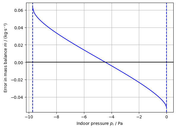
Figure 3. Residual of mass balance equation in the dolain of pressure variation (without wind effect).
Numerical solution#
Alternatively, the solution to the equation
can be found numerically.
np.mean([pi_min, pi_max])
-4.860799999999998
fsolve(f, np.mean([pi_min, pi_max]))
array([-4.44919771])
# numerical solution
root = fsolve(f, np.mean([pi_min, pi_max]))
root = float(root[0])
print(f"pᵢ = {root:.2f} Pa")
pᵢ = -4.45 Pa
Check the mass balance#
By knowing the indoor pressure \(p_i\), the mass flow rates \(\dot m_{ni}\), \(\dot m_{si}\) and \(\dot m_{ic}\) can be found and the mass balance
checked.
# verification of mass balance, kg/s
mn = ρo * Ko * (Pdn - root)**no
ms = ρo * Ko * (Pds - root)**no
mc = ρi * Kc * (root + Psi - Pdc - Pso)**nc
print("Check mass balance:")
print(f"mass flow: north: {2 * mn:.3f} kg/s, south: {2 * ms:.3f} kg/s")
print(f"mass flow chimney: {mc:.3f} kg/s")
print(f"error in mass flow balance: {2 * mn + 2 * ms - mc:.6f} kg/s\n")
Check mass balance:
mass flow: north: 0.019 kg/s, south: 0.019 kg/s
mass flow chimney: 0.038 kg/s
error in mass flow balance: 0.000000 kg/s
Considering the wind effect#
Dynamic pressure#
The dynamic pressures are:
\(P_{dn} = C_{pn} \, \frac{1}{2} \, \rho_o \,v^2\) - north face
\(P_{ds} = C_{ps} \, \frac{1}{2} \, \rho_o \, v^2\) - south face
\(P_{dc} = C_{pc} \, \frac{1}{2} \, \rho_o \, v^2\) - chimney
v = 18 * 1000 / 3600            # m/s, wind speed

# dynamic pressures, Pa
Pdn = Cpn * 0.5 * ρo * v**2     # north face
Pds = Cps * 0.5 * ρo * v**2     # south face
Pdc = Cpc * 0.5 * ρo * v**2     # chimney
Domain of variation of indoor pressure#
The domain of variation of \(p_i\) in order to have the flows shown in Figure 1 is:
pi_min, pi_max = Pdc + Pso - Psi, min(Pdn, Pds)
print(f"Pressure domain with wind: {pi_min:.2f} Pa < pi < {pi_max:.2f} Pa")
Pressure domain with wind: -21.23 Pa < pi < -9.04 Pa
Graphical solution of nolinear equation for indoor pressure#
The solution of this non-linear equation can be found graphically (Figure 4).
# plot error in mass balance
pi = np.linspace(pi_min, pi_max, 100)

fig, ax = plt.subplots()

ax.plot(pi, f(pi), 'g')
ax.axvline(x=pi_min, color='g', **{'linestyle': 'dashed'})
ax.axvline(x=pi_max, color='g', **{'linestyle': 'dashed'})
ax.axhline(color='k')

ax.set_ylabel(r'Error in mass balance, $\dot{m}$ / (kg·s⁻¹)')
ax.set_xlabel(r'Indoor pressure, $p_i$ / Pa')
ax.grid()
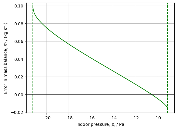
Figure 4. Residual of mass balance equation in the domain of pressure variation (with wind effect).
Numerical solution#
Alternatively, the solution to the equation
can be found numerically.
# numerical solution
root = fsolve(f, np.mean([pi_min, pi_max]))
print(f"pᵢ = {root[0]:.2f} Pa")
pᵢ = -10.50 Pa
Check the mass balance#
By knowing the indoor pressure \(p_i\), the mass flow rates \(\dot m_{ni}\), \(\dot m_{si}\) and \(\dot m_{ic}\) can be found and the mass balance
checked.
mn = ρo * Ko * (Pdn - root)**no
ms = ρo * Ko * (Pds - root)**no
mc = ρi * Kc * (root - (Pdc + Pso - Psi))**nc
mn2 = 2 * mn[0]
ms2 = 2 * ms[0]
mc = mc[0]
m_error = mn2 + ms2 - mc
print("Check mass balance:")
print(f"mass flow: north: {mn2:.3f} kg/s, south: {ms2:.3f} kg/s")
print(f"mass flow chimney: {mc:.3f} kg/s")
print(f"error in mass flow balance: {m_error:.6f} kg/s")
Check mass balance:
mass flow: north: 0.045 kg/s, south: 0.009 kg/s
mass flow chimney: 0.054 kg/s
error in mass flow balance: 0.000000 kg/s
References#
B. Rock, S.J. Emmerich, S. Taylor (2017) F16 Ventilation and Infiltration in ASHRAE Fundamentals Handbook, ISBN 10: 1939200598 ISBN 13: 978-1939200594